import rastereasy
Reduction of Dimension
1) Read the image
name_im='./data/demo/sentinel.tif'
names = {"NIR":8,"G":3,"CO" : 1,"SWIR2":11,"B": 2,"R":4,"RE1":5,"RE2":6,"RE3":7,"WA":9,"SWIR1":10,"SWIR3":12}
image=rastereasy.open(name_im,names=names)
image.info()
- Size of the image:
   - Rows (height): 1000
   - Cols (width): 1000
   - Bands: 12
- Spatial resolution: 10.0  meters / degree (depending on projection system)
- Central point latitude - longitude coordinates: (7.04099599, 38.39058840)
- Driver: GTiff
- Data type: int16
- Projection system: EPSG:32637
- Nodata: -32768.0

- Given names for spectral bands:
   {'CO': 1, 'B': 2, 'G': 3, 'R': 4, 'RE1': 5, 'RE2': 6, 'RE3': 7, 'NIR': 8, 'WA': 9, 'SWIR1': 10, 'SWIR2': 11, 'SWIR3': 12}
2) PCA
help(image.pca)
Help on method pca in module rastereasy:

pca(
    n_components=4,
    bands=None,
    random_state=None,
    dest_name=None,
    standardization=True,
    nb_points=1000
) method of rastereasy.Geoimage instance
    Perform PCA on the image data.

    This method computes a Principal Component Analysis (PCA) on selected image bands.

    Parameters
    ----------
    n_components : int, optional
        Number of components to keep (if None, all components are kept).
        Default is 4.
    bands : list of str or None, optional
        List of bands to use. If None, all bands are used.
        Default is None.
    random_state : int or None, optional
        Random seed for reproducible results. If None, results may vary between runs.
        Default is RANDOM_STATE (defined globally).
    dest_name : str, optional
        Path to save the decomposition. If None, the image is not saved.
        Default is None.
    standardization : bool, optional
        Whether to standardize bands before PCA (recommended).
        Default is True.
    nb_points : int or None, optional
        Number of random points to sample for PCA computation. If None,
        all valid pixels are used (may be slow for large images).
        Default is 1000.

    Returns
    -------
    Geoimage
        A new Geoimage containing the PCA bands.
    tuple
        A tuple (pca_model, scaler) to reuse the transformation on other images.

    Examples
    --------
    >>> # Basic PCA with 5 components
    >>> pca, (pca_model, scaler) = image.pca(n_components=5)
    >>> pca.visu(colorbar=True, cmap='viridis')

    >>> # PCA only on specific bands and save result
    >>> pca, (pca_model, scaler) = image.pca(
    ...     n_components=3, bands=["NIR", "Red", "Green"],
    ...     dest_name="pca.tif")

    >>> # Apply the same model to another image
    >>> other_pca = other_image.transform((pca_model, scaler))

    Notes
    -----
    - Standardization is recommended, especially when bands have different ranges.
    - The returned (pca_model, scaler) can be reused to project other images into the same PCA space.
2.1) PCA on the entire image
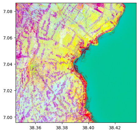
pca, pca_model = image.pca(n_components=3, nb_points=None)
pca.colorcomp()

pca.info()
- Size of the image:
   - Rows (height): 1000
   - Cols (width): 1000
   - Bands: 3
- Spatial resolution: 10.0  meters / degree (depending on projection system)
- Central point latitude - longitude coordinates: (7.04099599, 38.39058840)
- Driver: GTiff
- Data type: float64
- Projection system: EPSG:32637
- Nodata: -32768.0

- Given names for spectral bands:
   {'PCA_1': 1, 'PCA_2': 2, 'PCA_3': 3}
2.2) Applying the model to another image
image2=rastereasy.open('/Users/corpetti/Enseignement/2025-2026/TP_moustiques/im.tif', history=True)
help(image2.transform)
Help on method transform in module rastereasy:

transform(model, bands=None) method of rastereasy.Geoimage instance
    Apply a projection model  (PCA, tSNE, ...) to the image.

    This method applies a projection model (such as one created by pca())
    to the image data, creating a new   image.

    Parameters
    ----------
    model : scikit model or tuple
        If tuple, it must containi (data_model, scaler) where:
        - data_model: A trained scikit-learn model with a transform() method
        - scaler: The scaler used for standardization (or None if not used)
    bands : list of str or None, optional
        List of bands to use as input for the model. If None, all bands are used.
        Default is None.

    Returns
    -------
    Geoimage
        A new Geoimage containing the model output

    Examples
    --------
    >>> # Train a model on one image and apply to another
    >>> pca, model = reference_image.pca(n_components=5)
    >>> new_projection = target_image.transform(model)
    >>> new_projection.visu(colorbar=True, cmap='viridis')
    >>>
    >>> # Train on specific bands and apply to the same bands
    >>> _, model = image.pca(bands=["NIR", "Red"], n_components=3)
    >>> result = image.transform(model, bands=["NIR", "Red"])
    >>> result.save("pca.tif")
    >>>
    >>> # Apply a RF model trained of other data to a Geoimage
    >>> from sklearn.decomposition import PCA
    >>> clf = PCA(n_components=2, random_state=0)
    >>> clf.fit(X, y)
    >>> result = image.transform(clf)


    Notes
    -----
    - The model must have been trained on data with the same structure as what it's being applied to (e.g., same number of bands)
    - If a scaler was used during training, it will be applied before prediction
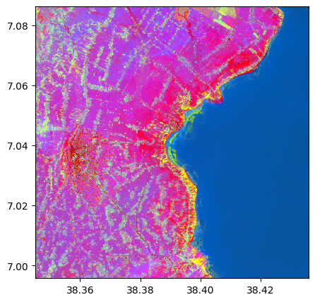
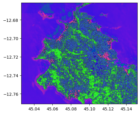
image2.colorcomp()
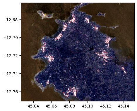
im_test_pca = image2.transform(pca_model)
im_test_pca.colorcomp()
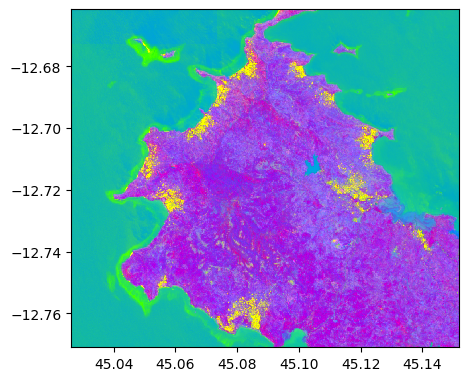
im_test_pca.info()
- Size of the image:
   - Rows (height): 1211
   - Cols (width): 1362
   - Bands: 3
- Spatial resolution: 10.0  meters / degree (depending on projection system)
- Central point latitude - longitude coordinates: (-12.71625261, 45.08894774)
- Driver: GTiff
- Data type: float64
- Projection system: EPSG:32738
- Nodata: -32768.0

- Given names for spectral bands:
   {'1': 1, '2': 2, '3': 3}

--- History of modifications---
[2025-12-06 09:29:21] - Created image from data array
[2025-12-06 09:29:21] - Created using transformation model: PCA
2.3) PCA on on selected bands
pca, pca_model = image.pca(n_components=3, nb_points=2000)
pca.colorcomp()
# Without standardization
pca, pca_model = image.pca(n_components=3, nb_points=2000, standardization=False)
pca.colorcomp()
# Only on some bands
pca, pca_model = image.pca(n_components=3, nb_points=2000, standardization=False, bands=['R','G','B','NIR'])
pca_model[0].explained_variance_
array([1873004.28292394, 133181.78089014, 4896.03373421])
pca.colorcomp()
2) LLE
help(image.lle)
Help on method lle in module rastereasy:

lle(
    n_components=2,
    n_neighbors=8,
    bands=None,
    nb_points=5000,
    standardization=True,
    dest_name=None,
    random_state=None,
    **kwargs
) method of rastereasy.Geoimage instance
    Perform Locally Linear Embedding (LLE) on the image data.

    This method computes a Locally Linear Embedding reduction to unfold the
    manifold on which the pixel values lie. It's particularly useful for
    data with an intrinsic low-dimensional structure that is non-linear.

    Parameters
    ----------
    n_components : int, optional
        The number of coordinates for the manifold (target dimension).
        Default is 2.
    n_neighbors : int, optional
        Number of neighbors to consider for each point. This is a crucial
        parameter for LLE that significantly impacts the result.
        Default is 8.
    bands : list of str or None, optional
        List of bands to use for the computation. If None, all bands are used.
        Default is None.
    nb_points : int or None, optional
        Number of random pixels to sample for the LLE computation. Since LLE
        is computationally intensive, using a sample is highly recommended for
        large images. If None, all valid pixels are used.
        Default is 5000.
    standardization : bool, optional
        Whether to standardize bands before applying LLE (highly recommended).
        Default is True.
    dest_name : str or None, optional
        Path to save the resulting LLE image. If None, the image is not saved.
        Default is None.
    random_state : int or None, optional
        Random seed for pixel sampling and for the ARPACK solver, ensuring
        reproducible results.
        Default is RANDOM_STATE.
    **kwargs : dict, optional
        Additional keyword arguments to pass to the scikit-learn
        `LocallyLinearEmbedding` function, such as `method` ('standard',
        'modified', 'hessian', 'ltsa'), `reg`, or `eigen_solver`.

    Returns
    -------
    Geoimage
        A new Geoimage instance containing the LLE components as bands.
    tuple
        A tuple (lle_model, scaler) containing the fitted LLE model and the
        scaler, which can be used to transform other images.

    Examples
    --------
    >>> # Basic LLE with 2 components
    >>> lle_img, (lle_model, scaler) = image.lle(n_components=2)
    >>> lle_img.visu(cmap='viridis')

    >>> # LLE with more neighbors on specific bands and save the result
    >>> lle_img, _ = image.lle(
    ...     n_components=3,
    ...     n_neighbors=20,
    ...     bands=["NIR", "Red", "Green"],
    ...     dest_name="lle_result.tif"
    ... )

    >>> # Apply the same LLE model to another image
    >>> other_image_lle = other_image.transform((lle_model, scaler))

    Notes
    -----
    - LLE is computationally more expensive than PCA. Using a subset of pixels
      via `nb_points` is strongly advised for large rasters.
    - The choice of `n_neighbors` is critical. A value too small may fail to
      capture the underlying manifold, while a value too large may over-smooth it.
    - The returned (lle_model, scaler) tuple can be used to project other images
      into the same embedding space, assuming they lie on the same manifold.
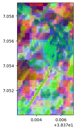
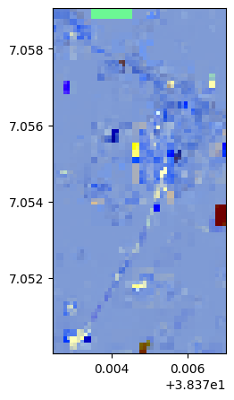
2.1) LLE on the entire image
# Read only a subset of the image since TSNE can be long
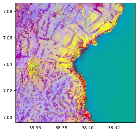
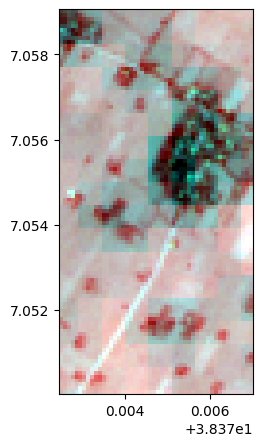
image=rastereasy.open(name_im,names=names, area=((300,400),(300,350)), history=True)
image.colorcomp()
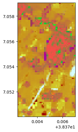
lle, lle_model = image.lle(n_components=3, n_neighbors= 12, nb_points=None)
lle.colorcomp()
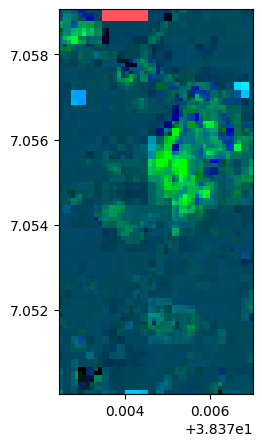
lle.info()
- Size of the image:
   - Rows (height): 100
   - Cols (width): 50
   - Bands: 3
- Spatial resolution: 10.0  meters / degree (depending on projection system)
- Central point latitude - longitude coordinates: (7.05454580, 38.37472999)
- Driver: GTiff
- Data type: float64
- Projection system: EPSG:32637
- Nodata: -32768.0

- Given names for spectral bands:
   {'LLE_1': 1, 'LLE_2': 2, 'LLE_3': 3}

--- History of modifications---
[2025-12-06 09:29:23] - Created image from data array
[2025-12-06 09:29:23] - Created using transformation model: LocallyLinearEmbedding
[2025-12-06 09:29:23] - Changed band names
[2025-12-06 09:29:23] - Created using LLE with 3 components
2.2) Applying the model to another image
image2=rastereasy.open('/Users/corpetti/Enseignement/2025-2026/TP_moustiques/im.tif', history=True)
help(image2.transform)
Help on method transform in module rastereasy:

transform(model, bands=None) method of rastereasy.Geoimage instance
    Apply a projection model  (PCA, tSNE, ...) to the image.

    This method applies a projection model (such as one created by pca())
    to the image data, creating a new   image.

    Parameters
    ----------
    model : scikit model or tuple
        If tuple, it must containi (data_model, scaler) where:
        - data_model: A trained scikit-learn model with a transform() method
        - scaler: The scaler used for standardization (or None if not used)
    bands : list of str or None, optional
        List of bands to use as input for the model. If None, all bands are used.
        Default is None.

    Returns
    -------
    Geoimage
        A new Geoimage containing the model output

    Examples
    --------
    >>> # Train a model on one image and apply to another
    >>> pca, model = reference_image.pca(n_components=5)
    >>> new_projection = target_image.transform(model)
    >>> new_projection.visu(colorbar=True, cmap='viridis')
    >>>
    >>> # Train on specific bands and apply to the same bands
    >>> _, model = image.pca(bands=["NIR", "Red"], n_components=3)
    >>> result = image.transform(model, bands=["NIR", "Red"])
    >>> result.save("pca.tif")
    >>>
    >>> # Apply a RF model trained of other data to a Geoimage
    >>> from sklearn.decomposition import PCA
    >>> clf = PCA(n_components=2, random_state=0)
    >>> clf.fit(X, y)
    >>> result = image.transform(clf)


    Notes
    -----
    - The model must have been trained on data with the same structure as what it's being applied to (e.g., same number of bands)
    - If a scaler was used during training, it will be applied before prediction
image2.colorcomp()
im_test_lle = image2.transform(lle_model)
im_test_lle.colorcomp()
im_test_lle.info()
- Size of the image:
   - Rows (height): 1211
   - Cols (width): 1362
   - Bands: 3
- Spatial resolution: 10.0  meters / degree (depending on projection system)
- Central point latitude - longitude coordinates: (-12.71625261, 45.08894774)
- Driver: GTiff
- Data type: float64
- Projection system: EPSG:32738
- Nodata: -32768.0

- Given names for spectral bands:
   {'1': 1, '2': 2, '3': 3}

--- History of modifications---
[2025-12-06 09:30:21] - Created image from data array
[2025-12-06 09:30:21] - Created using transformation model: LocallyLinearEmbedding
2.3) LLE on on selected bands
lle, lle_model = image.lle(n_components=3, nb_points=8000)
lle.colorcomp()
# Without standardization
lle, lle_model = image.lle(n_components=3, nb_points=2000, standardization=False)
lle.colorcomp()
# Only on some bands
lle, lle_model = image.lle(n_components=3, nb_points=2000, standardization=False, bands=['R','G','B','NIR'])
lle.colorcomp()
3) TSNE
help(image.tsne)
Help on method tsne in module rastereasy:

tsne(
    n_components=4,
    perplexity=5,
    bands=None,
    random_state=None,
    dest_name=None,
    standardization=True
) method of rastereasy.Geoimage instance
    Perform TSNE on the image data.

    This method computes a t-distributed Stochastic Neighbor Embeddings (tSNE) on selected image bands.

    Parameters
    ----------
    n_components : int, optional
        Number of components to keep (if None, all components are kept).
        Default is 4.
    perplexity : int, optional
        Perplexity in TSNE. It is related to the number of nearest neighbors
           that is used in other manifold learning algorithms.
        Default is 4.
    bands : list of str or None, optional
        List of bands to use. If None, all bands are used.
        Default is None.
    random_state : int or None, optional
        Random seed for reproducible results. If None, results may vary between runs.
        Default is RANDOM_STATE (defined globally).
    dest_name : str, optional
        Path to save the decomposition. If None, the image is not saved.
        Default is None.
    standardization : bool, optional
        Whether to standardize bands before PCA (recommended).
        Default is True.

    Returns
    -------
    Geoimage
        A new Geoimage containing the TSNE bands.
    tuple
        A tuple (tsne_model, scaler) to reuse the transformation on other images.

    Examples
    --------
    >>> # Basic TSNE with 5 components
    >>> tsne = image.tsne(n_components=5, perplexity = 5)
    >>> tsne.visu(colorbar=True, cmap='viridis')

    >>> # TSNE only on specific bands and save result
    >>> tsne = image.tsne(
    ...     n_components=3, , perplexity = 3, bands=["NIR", "Red", "Green"],
    ...     dest_name="tsne.tif")


    Notes
    -----
    - Standardization is recommended, especially when bands have different ranges.
    - The returned (tsne_model, scaler) can be reused to project other images into the same PCA space.
    - Unlike PCA, here we apply TSNE to the entire image. The model can not be applied to other ones
3.1) TSNE on the entire image
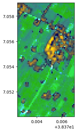
# Read only a subset of the image since TSNE can be long
image=rastereasy.open(name_im,names=names, area=((300,400),(300,350)), history=True)
image.colorcomp()

tsnei = image.tsne(n_components=3,  perplexity=10, bands=['R','G','RE2','SWIR1','NIR'])
tsnei.info()
- Size of the image:
   - Rows (height): 100
   - Cols (width): 50
   - Bands: 3
- Spatial resolution: 10.0  meters / degree (depending on projection system)
- Central point latitude - longitude coordinates: (7.05454580, 38.37472999)
- Driver: GTiff
- Data type: float32
- Projection system: EPSG:32637
- Nodata: -32768.0

- Given names for spectral bands:
   {'TSNE_1': 1, 'TSNE_2': 2, 'TSNE_3': 3}

--- History of modifications---
[2025-12-06 09:30:37] - Created image from data array
[2025-12-06 09:30:37] - Changed band names
[2025-12-06 09:30:37] - Created using TSNE with 3 components
	 Using bands: ['R', 'G', 'RE2', 'SWIR1', 'NIR']
tsnei.colorcomp()