import rastereasy

Adapting spectral bands with optimal transport

Read images, info and plot them

image1=rastereasy.Geoimage('./data/demo/source.tif')
image2=rastereasy.Geoimage('./data/demo/target.tif')
image1.info()
image2.info()

- Size of the image:
   - Rows (height): 1000
   - Cols (width): 1000
   - Bands: 3
- Spatial resolution: 10.0  meters / degree (depending on projection system)
- Central point latitude - longitude coordinates: (41.88007631, -4.51648135)
- Driver: GTiff
- Data type: int16
- Projection system: EPSG:32630
- Nodata: -32768.0

- Given names for spectral bands: 
   {'1': 1, '2': 2, '3': 3}


- Size of the image:
   - Rows (height): 1000
   - Cols (width): 1000
   - Bands: 3
- Spatial resolution: 10.000728597449909  meters / degree (depending on projection system)
- Central point latitude - longitude coordinates: (41.88003619, -4.51641528)
- Driver: GTiff
- Data type: uint16
- Projection system: EPSG:32630

- Given names for spectral bands: 
   {'1': 1, '2': 2, '3': 3}

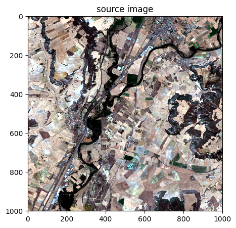
image1.colorcomp(extent='pixel', title='source image')
image2.colorcomp(extent='pixel', title = 'target image')

<Figure size 640x480 with 0 Axes>

<Figure size 640x480 with 0 Axes>

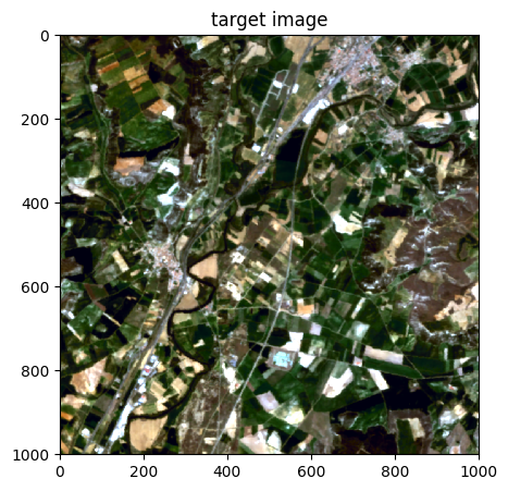
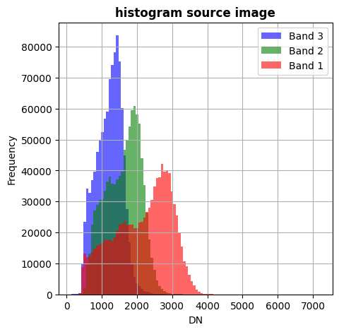
image1.hist(superpose=True, title='histogram source image')
image2.hist(superpose=True, title='histogram target image')

<Figure size 640x480 with 0 Axes>

<Figure size 640x480 with 0 Axes>

Domain adaptation. Two possibilities :

1. return an adapted image (image1.adapt function)

2. directly modify the image (image1.adapt function with inplace=True option)

help(image1.adapt)

Help on method adapt in module rastereasy.rastereasy:

adapt(imt, tab_source=None, nb=1000, mapping='gaussian', reg_e=0.1, mu=1.0, eta=0.01, bias=False, max_iter=20, verbose=True, sigma=1, inplace=False) method of rastereasy.rastereasy.Geoimage instance
    Adjust spectral characteristics to match a target image.
    
    This method adapts the spectral characteristics of the current image to match
    those of a target image using optimal transport methods. This is useful for
    harmonizing images from different sensors or acquisitions.
    
    Parameters
    ----------
    imt : Geoimage or numpy.ndarray
        Target image serving as a reference for spectral adjustment,
        or a NumPy array of shape (N, bands) containing N spectral samples.
    tab_source : numpy.ndarray, optional
        Required if `imt` is a NumPy array. Must be an array of shape (M, bands)
        containing spectral samples from the source image.
    nb : int, optional
        Number of random samples used to train the transport model.
        Default is 1000.
    mapping : str, optional
        Optimal transport method to use:
        - 'emd': Earth Mover's Distance (simplest)
        - 'sinkhorn': Sinkhorn transport with regularization (balanced)
        - 'mappingtransport': Mapping-based transport (flexible)
        - 'gaussian': Transport with Gaussian assumptions (default, robust)
        Default is 'gaussian'.
    reg_e : float, optional
        Regularization parameter for Sinkhorn transport.
        Default is 1e-1.
    mu : float, optional
        Regularization parameter for mapping-based methods.
        Default is 1e0.
    eta : float, optional
        Learning rate for mapping-based transport methods.
        Default is 1e-2.
    bias : bool, optional
        Whether to add a bias term to the transport model.
        Default is False.
    max_iter : int, optional
        Maximum number of iterations for iterative transport methods.
        Default is 20.
    verbose : bool, optional
        Whether to display progress information.
        Default is True.
    sigma : float, optional
        Standard deviation used for Gaussian transport methods.
        Default is 1.
    inplace : bool, default False
        If False, return a copy. Otherwise, do the adaptation in place and return None.
    
    Returns
    -------
        The image with adapted spectral characteristics or None if `inplace=True`
    
    Examples
    --------
    >>> # Basic spectral adaptation
    >>> image_adapt = image1.adapt(image2)
    >>> image_adapt.visu()  # Now spectrally similar to image2
    >>>
    >>> # Use specific transport method
    >>> image_adapt = image1.adapt(image2, mapping='sinkhorn', reg_e=0.01)
    >>> image_adapt.save("adapted_image.tif")
    >>>
    >>> # Adaptation using sample arrays
    >>> adapted_image = image1.adapt(tab_target, tab_source = tab_source, mapping='sinkhorn', reg_e=0.01)
    >>>
    >>> # Basic spectral adaptation and modify inplace the image
    >>> image1.adapt(image2, inplace=True)
    >>> image1.visu()  # Now spectrally similar to image2
    
    Notes
    -----
    - This method is useful for:
        - Harmonizing multi-sensor data
        - Matching images acquired under different conditions
        - Preparing time-series data for consistent analysis
    - Different mapping methods have different characteristics:
        - 'emd': Most accurate but slowest
        - 'sinkhorn': Good balance between accuracy and speed
        - 'mappingtransport': Flexible and can handle complex transformations
        - 'gaussian': Fastest and works well for most cases

1) Adaptation

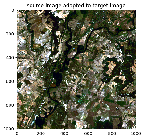
image1_adapted = image1.adapt(image2,mapping='emd')

Fitting transport model using emd method...
Transforming data...
Adaptation complete.

image1_adapted.colorcomp(title='source image adapted to target image',extent='pixel')
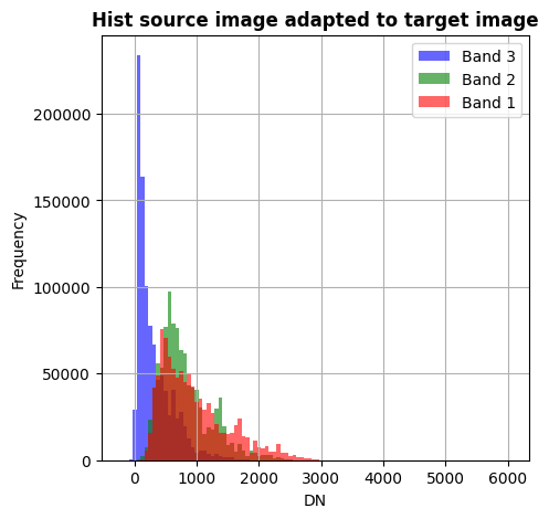
image1_adapted.hist(superpose=True,title='Hist source image adapted to target image')

<Figure size 640x480 with 0 Axes>

<Figure size 640x480 with 0 Axes>

2) By modifying the image directly inplace=True option

image1.colorcomp(title='image 1 before adaptation',extent='pixel')
image1.hist(superpose=True,xmin=0,xmax=5000,title = 'hist image 1 before adaptation')

<Figure size 640x480 with 0 Axes>

<Figure size 640x480 with 0 Axes>

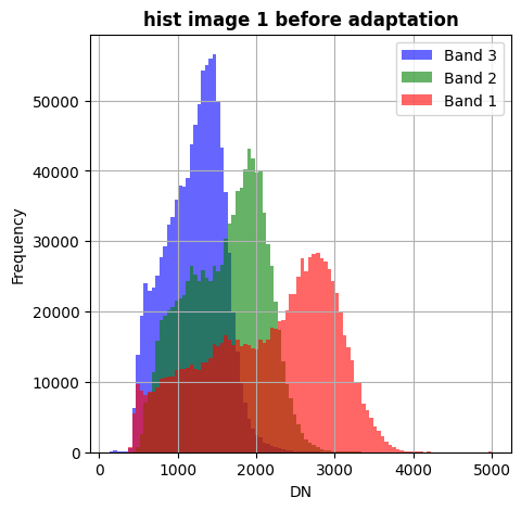
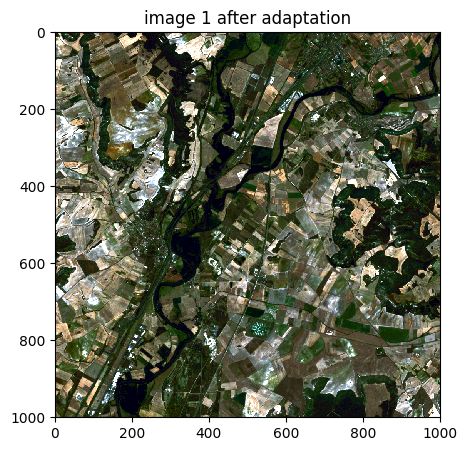
image1.adapt(image2,mapping='emd',inplace=True)

Fitting transport model using emd method...
Transforming data...
Adaptation complete.

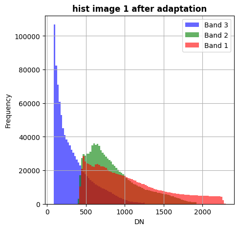
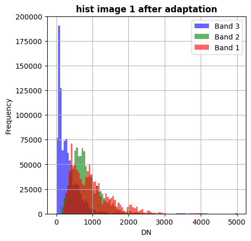
image1.colorcomp(title='image 1 after adaptation',extent='pixel')
image1.hist(superpose=True,xmin=0,xmax=5000,title = 'hist image 1 after adaptation')

<Figure size 640x480 with 0 Axes>

<Figure size 640x480 with 0 Axes>

2) By manually selecting the samples

image1=rastereasy.Geoimage('./data/demo/source.tif')
image2=rastereasy.Geoimage('./data/demo/target.tif')
image1.info()
image2.info()

- Size of the image:
   - Rows (height): 1000
   - Cols (width): 1000
   - Bands: 3
- Spatial resolution: 10.0  meters / degree (depending on projection system)
- Central point latitude - longitude coordinates: (41.88007631, -4.51648135)
- Driver: GTiff
- Data type: int16
- Projection system: EPSG:32630
- Nodata: -32768.0

- Given names for spectral bands: 
   {'1': 1, '2': 2, '3': 3}


- Size of the image:
   - Rows (height): 1000
   - Cols (width): 1000
   - Bands: 3
- Spatial resolution: 10.000728597449909  meters / degree (depending on projection system)
- Central point latitude - longitude coordinates: (41.88003619, -4.51641528)
- Driver: GTiff
- Data type: uint16
- Projection system: EPSG:32630

- Given names for spectral bands: 
   {'1': 1, '2': 2, '3': 3}

samples_source,_,_=image1.plot_spectra()

samples_target,_,_=image2.plot_spectra()

print('size of sample source = ',len(samples_source))
print('size of sample target = ',len(samples_target))

size of sample source =  63
size of sample target =  51

import numpy as np

image1_adapted = image1.adapt(np.array(samples_target),np.array(samples_source),mapping='sinkhorn')

Fitting transport model using sinkhorn method...
Transforming data...
Adaptation complete.

image1_adapted.colorcomp(extent='pixel', title = 'image 1 after adaptation')

<Figure size 640x480 with 0 Axes>

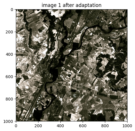
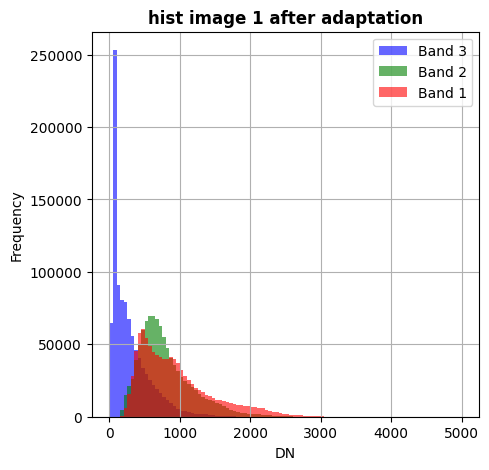
image2.hist(superpose=True,xmin=0,xmax=5000,title = 'hist image 1 after adaptation')
image1_adapted.hist(superpose=True,xmin=0,xmax=5000,title = 'hist image 1 after adaptation')

<Figure size 640x480 with 0 Axes>

<Figure size 640x480 with 0 Axes>