Compute features and perform Machine Learning

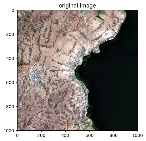
1. In this example, we load a SENTINEL image and compute some features on this image :

• Gaussian filters of RGB NIR bands

• NDVI and NDVI filtered with Gaussian & Laplacian

2. Then, we load a Field data tif image that contains the different classes (only two in our situation).

3. We extract two numpy that are required in a random forest (with scikit)

4. We apply the model to the entire image

import rastereasy

1) Process sentinel image

1.1) Read image

name_im='./data/demo/sentinel.tif'
names = {"CO" : 1,"B": 2,"G":3,"R":4,"RE1":5,"RE2":6,"RE3":7,"NIR":8,"WA":9,"SWIR1":10,"SWIR2":11,"SWIR3":12}
image=rastereasy.Geoimage(name_im, names=names)
image.info()
image.colorcomp(bands=['R','G','B'], extent='pixel',title='original image')

- Size of the image:
   - Rows (height): 1000
   - Cols (width): 1000
   - Bands: 12
- Spatial resolution: 10.0  meters / degree (depending on projection system)
- Central point latitude - longitude coordinates: (7.04099599, 38.39058840)
- Driver: GTiff
- Data type: int16
- Projection system: EPSG:32637
- Nodata: -32768.0

- Given names for spectral bands: 
   {'CO': 1, 'B': 2, 'G': 3, 'R': 4, 'RE1': 5, 'RE2': 6, 'RE3': 7, 'NIR': 8, 'WA': 9, 'SWIR1': 10, 'SWIR2': 11, 'SWIR3': 12}

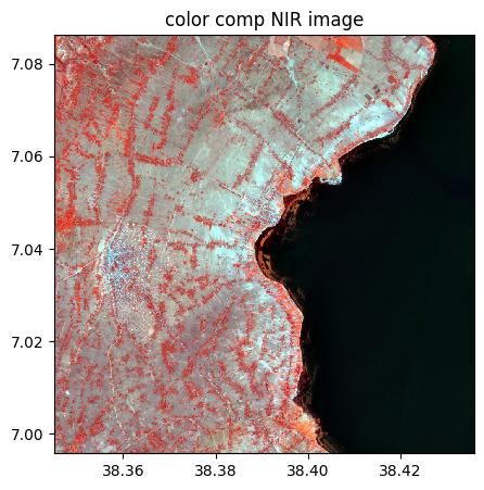
1.2) Extract R,G,B,NIR

rgbnir=image.select_bands(['R','G','B','NIR'])
rgbnir.info()
rgbnir.colorcomp(bands=['NIR','G','B'], title = 'color comp NIR image')

- Size of the image:
   - Rows (height): 1000
   - Cols (width): 1000
   - Bands: 4
- Spatial resolution: 10.0  meters / degree (depending on projection system)
- Central point latitude - longitude coordinates: (7.04099599, 38.39058840)
- Driver: GTiff
- Data type: int16
- Projection system: EPSG:32637
- Nodata: -32768.0

- Given names for spectral bands: 
   {'R': 1, 'G': 2, 'B': 3, 'NIR': 4}

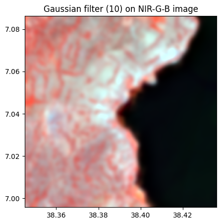
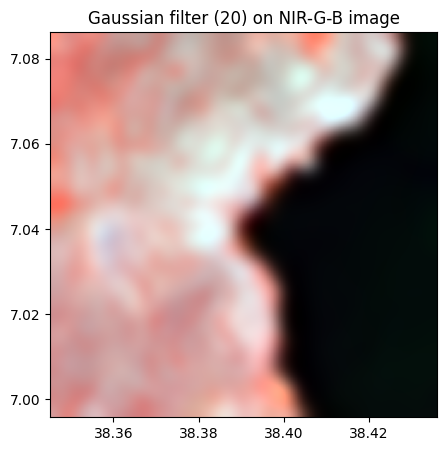
1.3) Compute gaussian filters with sigma=10 and sigma=20

# sigma = 10
rgbnir_10=rgbnir.filter(method="gaussian",sigma=10)
rgbnir_10.colorcomp(bands=['R','G','B'], title = 'Gaussian filter (10) on RGB image')
rgbnir_10.colorcomp(bands=['NIR','G','B'], title = 'Gaussian filter (10) on NIR-G-B image')

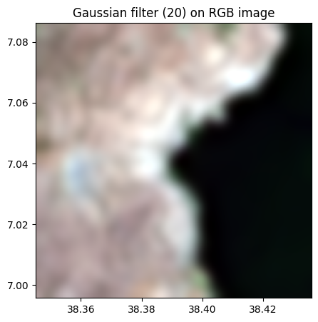
# sigma = 20
rgbnir_20=rgbnir.filter(method="gaussian",sigma=20)
rgbnir_20.colorcomp(bands=['R','G','B'], title = 'Gaussian filter (20) on RGB image')
rgbnir_20.colorcomp(bands=['NIR','G','B'], title = 'Gaussian filter (20) on NIR-G-B image')

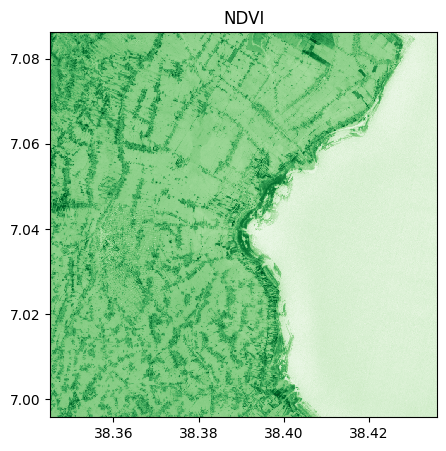
1.4) Compute NDVI and two filtered version (gaussian sigma=10 and sigma=20)

Extract R and NIR bands

r=rgbnir.select_bands('R')
nir=rgbnir.select_bands('NIR')

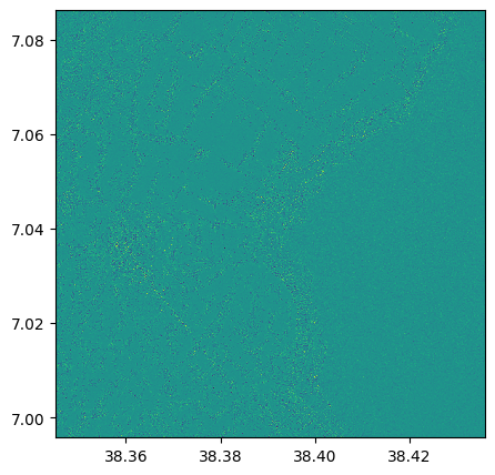
Compute and visu NDVI

ndvi=(nir-r)/(nir+r)
ndvi.visu(cmap='Greens', title="NDVI")
ndvi.info()

- Size of the image:
   - Rows (height): 1000
   - Cols (width): 1000
   - Bands: 1
- Spatial resolution: 10.0  meters / degree (depending on projection system)
- Central point latitude - longitude coordinates: (7.04099599, 38.39058840)
- Driver: GTiff
- Data type: float64
- Projection system: EPSG:32637
- Nodata: nan

- Given names for spectral bands: 
   {'NIR': 1}

# As we can see, the name associated is the name of the 1st band involved in the operation
# For more consistency, we can change the name with :
ndvi.change_names({'NDVI':1})
ndvi.info()

- Size of the image:
   - Rows (height): 1000
   - Cols (width): 1000
   - Bands: 1
- Spatial resolution: 10.0  meters / degree (depending on projection system)
- Central point latitude - longitude coordinates: (7.04099599, 38.39058840)
- Driver: GTiff
- Data type: float64
- Projection system: EPSG:32637
- Nodata: nan

- Given names for spectral bands: 
   {'NDVI': 1}

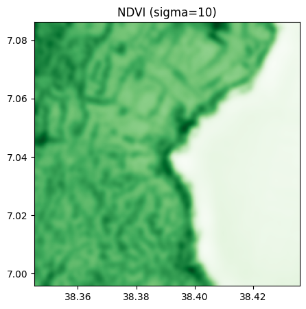
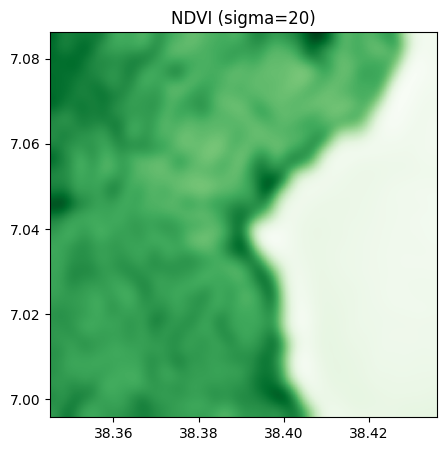
Gaussian filter of NDVI

# sigma = 10 and 20
ndvi_10=ndvi.filter(method="gaussian",sigma=10)
ndvi_20=ndvi.filter(method="gaussian",sigma=20)
ndvi_10.visu(cmap='Greens', title="NDVI (sigma=10)")
ndvi_20.visu(cmap='Greens', title="NDVI (sigma=20)")

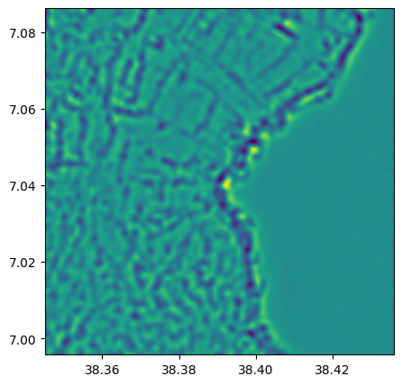
Laplacian filter of NDVI

laplace_1=ndvi.filter(method = 'laplace')
laplace_1.visu()
laplace_2=ndvi.filter(method = 'laplace', pre_smooth_sigma=10)
laplace_2.visu()

2) Stack all features

We can now stack all features, in rgbnir, rgbnir_10, rgbnir_20, ndvi, ndvi_10, ndvi_20, laplace_1, laplace_2

im_features=rgbnir.stack(rgbnir_10).stack(rgbnir_20).stack(ndvi).stack(ndvi_10).stack(ndvi_20).stack(laplace_1).stack(laplace_2)
im_features.info()

- Size of the image:
   - Rows (height): 1000
   - Cols (width): 1000
   - Bands: 17
- Spatial resolution: 10.0  meters / degree (depending on projection system)
- Central point latitude - longitude coordinates: (7.04099599, 38.39058840)
- Driver: GTiff
- Data type: float64
- Projection system: EPSG:32637
- Nodata: -32768.0

- Given names for spectral bands: 
   {'R_1_1_1': 1, 'G_1_1_1': 2, 'B_1_1_1': 3, 'NIR_1_1_1': 4, 'R_2_1_1': 5, 'G_2_1_1': 6, 'B_2_1_1': 7, 'NIR_2_1_1': 8, 'R_1_1': 9, 'G_1_1': 10, 'B_1_1': 11, 'NIR_1_1': 12, 'NDVI_1_1': 13, 'NDVI_2_1': 14, 'NDVI_1': 15, 'NDVI_2': 16, 'NDVI': 17}

As we can see, names are adapted. For more clarity, we can

• change the names of each individual features (ex: ndvi_10.change_names({'NDVI_10':1}) to make the naming of stacks

• Reformat names with im_features.reset_names()

We decide here the second solution

im_features.reset_names()
im_features.info()

- Size of the image:
   - Rows (height): 1000
   - Cols (width): 1000
   - Bands: 17
- Spatial resolution: 10.0  meters / degree (depending on projection system)
- Central point latitude - longitude coordinates: (7.04099599, 38.39058840)
- Driver: GTiff
- Data type: float64
- Projection system: EPSG:32637
- Nodata: -32768.0

- Given names for spectral bands: 
   {'1': 1, '2': 2, '3': 3, '4': 4, '5': 5, '6': 6, '7': 7, '8': 8, '9': 9, '10': 10, '11': 11, '12': 12, '13': 13, '14': 14, '15': 15, '16': 16, '17': 17}

3) Standardize the features

It is in general useful to standardize data for ML algorithms

im_features_std,scaler  = im_features.standardize()
# Check that mean is 0 and std 1
print(im_features_std.mean(axis='pixel'))
print(im_features_std.std(axis='pixel'))

[ 1.25112365e-16 -7.51185780e-17 -5.80371307e-17 -5.67297320e-17
  2.00537897e-14  3.86009447e-15  2.83656618e-14 -2.11864517e-14
 -4.87677312e-14  8.21022468e-14  6.18409217e-14  4.41988277e-14
 -3.19445860e-13  9.11597908e-15  1.28763418e-14  2.05613304e-19
  1.24913413e-17]
[1. 1. 1. 1. 1. 1. 1. 1. 1. 1. 1. 1. 1. 1. 1. 1. 1.]

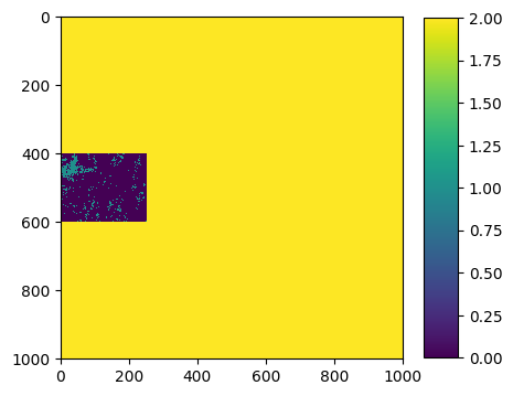
4) Read the classes data

name_data_classes = './data/demo/field_vegetation.tif'
ground_truth = rastereasy.Geoimage(name_data_classes)
ground_truth.visu(extent='pixel',colorbar=True)
ground_truth.info()

- Size of the image:
   - Rows (height): 1000
   - Cols (width): 1000
   - Bands: 1
- Spatial resolution: 10.0  meters / degree (depending on projection system)
- Central point latitude - longitude coordinates: (7.04099599, 38.39058840)
- Driver: GTiff
- Data type: uint8
- Projection system: EPSG:32637
- Nodata: 2.0

- Given names for spectral bands: 
   {'1': 1}

Here, we have 3 labels : 0,1,2:

• 0 corresponds to bare soils

• 1 corresponds to vegetation

• 2 corresponds to no data

We then have to extract only labels with 0 and 1 for the training (and not care with label 2).

To do this, we have the function rastereasy.extract_numpy_tables

4) Extract two numpy that are required in a scikit ML technique

scikitrequires (X,y) numpy tables:

• X being the data, of size (N x f) (N: number of data and f: number of features)

• y being the outputs, of size (N,) that contains the outputs (values, name of the class, …)

help(rastereasy.extract_numpy_tables)

Help on function extract_numpy_tables in module rastereasy.rastereasy:

extract_numpy_tables(data, outputs, label=None)
    Extract paired NumPy tables (features and outputs) for machine learning.
    
    This function converts raster data stored in `Geoimage` objects into two
    NumPy arrays: one containing the input features (X), and one containing
    the corresponding outputs/labels (y). Optionally, it can filter the
    dataset to only include samples corresponding to one or multiple label
    values.
    
    Parameters
    ----------
    data : Geoimage
        A `rastereasy.Geoimage` containing the input features
        (e.g., multispectral bands).
    outputs : Geoimage
        A `rastereasy.Geoimage` containing the outputs/labels
        (e.g., classes or quantitative values).
    label : int or list of int, optional (default=None)
        If provided, only the samples corresponding to this label value
        (or list of values) in `outputs` will be extracted.
    
    Returns
    -------
    X : numpy.ndarray
        Input feature table of shape (N, f), where
        N is the number of extracted samples and
        f is the number of features (bands).
    y : numpy.ndarray
        Output array of shape (N, ), containing the labels/outputs
        associated with each sample.
    
    Examples
    --------
    >>> # Extract all data/labels from two Geoimages
    >>> X, y = extract_numpy_tables(data, labels)
    
    >>> # Extract only the samples where label == 1
    >>> X, y = extract_numpy_tables(data, outputs, label=1)
    
    >>> # Extract only the samples with labels in [1, 3, 5]
    >>> X, y = extract_numpy_tables(data, outputs, label=[1, 3, 5])

# We are interested in labels 0 and 1 for training
X,y=rastereasy.extract_numpy_tables(im_features_std, ground_truth, label=[0,1])
print(X.shape)
print(y.shape)

(50000, 17)
(50000,)

5) Train our favorite ML algorithm

Now we can apply a ML algorithm on data. Here we use a random forest

Training

from sklearn.ensemble import RandomForestClassifier
clf = RandomForestClassifier(max_depth=2, random_state=0)
clf.fit(X, y)

RandomForestClassifier(max_depth=2, random_state=0)

In a Jupyter environment, please rerun this cell to show the HTML representation or trust the notebook.
On GitHub, the HTML representation is unable to render, please try loading this page with nbviewer.org.

6) Apply our favorite ML algorithm on a Geoimage

To apply the trained model on a Geoimage, we have the fonction predict

help(im_features_std.predict)

Help on method predict in module rastereasy.rastereasy:

predict(model, bands=None) method of rastereasy.rastereasy.Geoimage instance
    Apply a pre-trained machine learning model to the image.
    
    This method applies a machine learning model (such as one created by kmeans())
    to the image data, creating a new classified or transformed image.
    
    Parameters
    ----------
    model : scikit model or tuple
        If tuple, it must containi (ml_model, scaler) where:
        - ml_model: A trained scikit-learn model with a predict() method
        - scaler: The scaler used for standardization (or None if not used)
    bands : list of str or None, optional
        List of bands to use as input for the model. If None, all bands are used.
        Default is None.
    
    Returns
    -------
    Geoimage
        A new Geoimage containing the model output
    
    Examples
    --------
    >>> # Train a model on one image and apply to another
    >>> classified, model = reference_image.kmeans(n_clusters=5)
    >>> new_classified = target_image.predict(model)
    >>> new_classified.visu(colorbar=True, cmap='viridis')
    >>>
    >>> # Train on specific bands and apply to the same bands
    >>> _, model = image.kmeans(bands=["NIR", "Red"], n_clusters=3)
    >>> result = image.predict(model, bands=["NIR", "Red"])
    >>> result.save("classified.tif")
    >>>
    >>> # Apply a RF model trained of other data to a Geoimage
    >>> from sklearn.ensemble import RandomForestClassifier
    >>> clf = RandomForestClassifier(max_depth=2, random_state=0)
    >>> clf.fit(X, y)
    >>> result = image.predict(clf)
    
    
    Notes
    -----
    - The model must have been trained on data with the same structure as what it's being applied to (e.g., same number of bands)
    - If a scaler was used during training, it will be applied before prediction
    - This method is useful for:
    - Applying a classification model to new images
    - Ensuring consistent classification across multiple scenes
    - Time-series analysis with consistent classification

# As we can see in the help, we can apply it directly on the image with standardized bands
vegetation = im_features_std.predict(clf)
vegetation.visu()

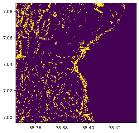
# We can apply it directly on the image without standardized bands, and give the scaler issued from standardization
vegetation = im_features.predict((clf,scaler))
vegetation.visu()