import rastereasy
Rastereasy
In rastereasy, one of the main class to deal with georeferenced images is Geoimage. It contains the main functions (for resampling, reprojection, stack, plotting, …). Let’s start by opening and plotting an image, some bands or making color compositions
Important for google colab
To use the interactive plotting features in Google Colab, a special two-step setup is required. Follow these steps in the exact order. Separating the commands into different cells and restarting the session is essential.
Step 1: Install Libraries
Run the following cell to install rastereasy and the necessary dependencies for interactive widgets.
!pip install rastereasy ipympl
from google.colab import output
output.enable_custom_widget_manager()
Step 2: Restart the Runtime
After the installation is complete, you must restart the runtime.
Go to the menu: Runtime > Restart runtime (or use the shortcut Ctrl+M).
Step 3: Run Your Code
After restarting, you can now enable the interactive mode and use the library in a new cell.
%matplotlib widget
import rastereasy
1) first step: open and visualize an image
# Check the help to initialize a `Geoimage` image
help(rastereasy.open)
Help on function open in module rastereasy:

open(filename, *args, **kwargs)
    Open a Geoimage object from a file or data array with metadata.

    Parameters
    ----------
    source_name : str, optional
        Path to a geoimage (.tif, .jp2) image file to load.
        If provided, the image data and metadata
        will be read from this file.
    meta_only : bool, optional
        If True, do not read the image but just
        the meta information (useful for image.info()).
    names : dict, optional
        Dictionary mapping band names to
        band indices (e.g., {'NIR': 1, 'R': 2, 'G': 3}).
        If not provided, bands will be
        named numerically ('1', '2', '3', ...).
    area : tuple, optional
        To read  only a window of the image
            If based on pixel coordinates, you must indicate
            - the row/col coordinades of
                    the north-west corner (deb_row,deb_col)
            - the row/col coordinades of
                    the south-east corner (end_row,end_col)
            in a tuple  `area = ((deb_row,end_row),(deb_col,end_col))`

            If based on latitude/longitude coordinates, you must indicate
            - the lat/lon coordinades of the north-west corner (lat1,lon1)
            - the lat/lon coordinades of the south-east corner (lat2,lon2)
            `area = ((lon1,lon2),(lat1,lat2))`
        If not provide, read the entire image
    extent : str, optional
        if `area` is given, precise if the coordinates
        are in pixels (extent = "pixel", default)
        or latitude/longitude (extent = "latlon")
    history : bool, optional
        Whether to track modification history for the image.
        Default is False.
    data : numpy.ndarray, optional
        Image data to initialize the object with.
        Must be provided with `meta`.
        Shape should be (bands, rows, cols).
    meta : dict, optional
        Metadata dictionary containing rasterio
        metadata fields (e.g., crs, transform).
        Required if `data` is provided.
    georef : bool, optional
        Whether the image is georeferenced.
        If None, will be determined from metadata.
    target_crs : str, optional
        Target coordinate reference system
        if reprojection is needed during loading.
        Default is "EPSG:4326".

    Attributes
    ----------
    image : numpy.ndarray
        The image data array with shape (bands, rows, cols).
    shape : tuple
        The dimensions of the image as (rows, cols).
    nb_bands : int
        The number of spectral bands in the image.
    resolution : float
        The spatial resolution of the image (pixel size in map units).
    names : dict
        Dictionary mapping band names to band indices.
    nodata : float or int
        Value used to represent no data or invalid pixels.

    Examples
    --------
    >>> # Read only meta information
    >>> img = rastereasy.open("landsat_image.tif",meta_only=True)
    >>> img.info()
    >>>
    >>> # Read an entire Geoimage from a file
    >>> img = rastereasy.open("landsat_image.tif")
    >>> img.info()
    >>>
    >>> # Read a window of a file from pixel coordinates
    >>> You must indicate
    >>>      - the row/col coordinades of
    >>>            the north-west corner (deb_row,deb_col)
    >>>      - the row/col coordinades of
    >>>            the south-east corner (end_row,end_col)
    >>> in a tuple  `((deb_row,end_row),(deb_col,end_col))`
    >>> img = rastereasy.open("landsat_image.tif", area=((200,500),(240,600)))
    >>> img.info()
    >>>
    >>> # Read a window of a file from lat/lon coordinates (parameter extent='latlon')
    >>> You must indicate
    >>>      - the lat/lon coordinades of the north-west corner (lat1,lon1)
    >>>      - the lat/lon coordinades of the south-east corner (lat2,lon2)
    >>> in a tuple  `((lon1,lon2),(lat1,lat2))`
    >>> img = rastereasy.open("landsat_image.tif", area=((38.36,38.41),(7.06,7.02)),extent='latlon'))
    >>> img.info()
    >>>
    >>> # Create a Geoimage from a NumPy array with metadata
    >>> meta = {'driver': 'GTiff', 'width': 100, 'height': 100, 'count': 3,
    >>> ...         'crs': CRS.from_epsg(4326), 'transform': Affine(0.1, 0, 0, 0, -0.1, 0)}
    >>> data = np.zeros((3, 100, 100))
    >>> img = rastereasy.open(data=data, meta=meta)
    >>>
    >>> # Create a Geoimage with custom band names
    >>> img = rastereasy.open("landsat_image.tif", names={'R': 1, 'G': 2, 'B': 3, 'NIR': 4})
    >>>
    >>> # Create a Geoimage with custom band names
    >>> img = rastereasy.open("landsat_image.tif", names={'R': 1, 'G': 2, 'B': 3, 'NIR': 4})
name_im='./data/demo/sentinel.tif'
Read basic information of the image, without open it (parameter meta_only=True)
image=rastereasy.open(name_im, meta_only=True)
# This is equivalent to
# image=rastereasy.Geoimage(name_im, meta_only=True)
image.info()
- Size of the image:
   - Rows (height): 1000
   - Cols (width): 1000
   - Bands: 12
- Spatial resolution: 10.0  meters / degree (depending on projection system)
- Central point latitude - longitude coordinates: (7.04099599, 38.39058840)
- Driver: GTiff
- Data type: int16
- Projection system: EPSG:32637
- Nodata: -32768.0

- Given names for spectral bands:
   {'1': 1, '2': 2, '3': 3, '4': 4, '5': 5, '6': 6, '7': 7, '8': 8, '9': 9, '10': 10, '11': 11, '12': 12}
Open the image and print information
image=rastereasy.open(name_im)
# This is equivalent to
# image=rastereasy.Geoimage(name_im)
image.info()
- Size of the image:
   - Rows (height): 1000
   - Cols (width): 1000
   - Bands: 12
- Spatial resolution: 10.0  meters / degree (depending on projection system)
- Central point latitude - longitude coordinates: (7.04099599, 38.39058840)
- Driver: GTiff
- Data type: int16
- Projection system: EPSG:32637
- Nodata: -32768.0

- Given names for spectral bands:
   {'1': 1, '2': 2, '3': 3, '4': 4, '5': 5, '6': 6, '7': 7, '8': 8, '9': 9, '10': 10, '11': 11, '12': 12}
As we can see, spectral bands car named '1', '2', ... in a dictionnary where the name is associated with its number in the image (from 1 to the number of bands).
Alternatively , we can give more explicit names to the spectral bands by specifying them :
# Alternatively, we can give names to bands
names = {"CO" : 1,"B": 2,"G":3,"R":4,"RE1":5,"RE2":6,"RE3":7,"NIR":8,"WA":9,"SWIR1":10,"SWIR2":11,"SWIR3":12}
image_names=rastereasy.open(name_im,names=names)
image_names.info()
# Note : this is equavalent to image.change_names(names)
- Size of the image:
   - Rows (height): 1000
   - Cols (width): 1000
   - Bands: 12
- Spatial resolution: 10.0  meters / degree (depending on projection system)
- Central point latitude - longitude coordinates: (7.04099599, 38.39058840)
- Driver: GTiff
- Data type: int16
- Projection system: EPSG:32637
- Nodata: -32768.0

- Given names for spectral bands:
   {'CO': 1, 'B': 2, 'G': 3, 'R': 4, 'RE1': 5, 'RE2': 6, 'RE3': 7, 'NIR': 8, 'WA': 9, 'SWIR1': 10, 'SWIR2': 11, 'SWIR3': 12}
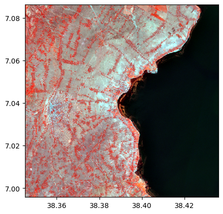
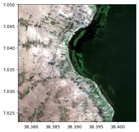
Create a color composite of image using bands 4, 3, and 2
image.colorcomp(['9', '3', '2'])
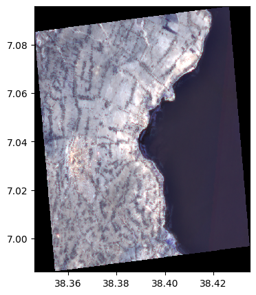
Create a color composite of image_names using bands R, G, and B and visualize it with a map on background
image_names.colorcomp(['R', 'G', 'B'], background='map')
2) Example of easy manipulations (resample, reproject. See dedicated examples for more details / options)
Resample the image to a resolution of 15 meters
image_resampled = image.resample(15)
image_resampled.info()
image.resample(15,inplace=True) # inplace=True : modify directly the image
image.info()
- Size of the image:
   - Rows (height): 666
   - Cols (width): 666
   - Bands: 12
- Spatial resolution: 15.015015015015013  meters / degree (depending on projection system)
- Central point latitude - longitude coordinates: (7.04097334, 38.39061114)
- Driver: GTiff
- Data type: int16
- Projection system: EPSG:32637
- Nodata: -32768.0

- Given names for spectral bands:
   {'1': 1, '2': 2, '3': 3, '4': 4, '5': 5, '6': 6, '7': 7, '8': 8, '9': 9, '10': 10, '11': 11, '12': 12}
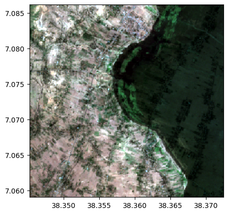
Reproject the image to the EPSG:27700 coordinate system
image_reproject = image.reproject("EPSG:27700")
image_reproject.info()
image_reproject.colorcomp()
- Size of the image:
   - Rows (height): 733
   - Cols (width): 733
   - Bands: 12
- Spatial resolution: 19.64992127401193  meters / degree (depending on projection system)
- Central point latitude - longitude coordinates: (7.04099917, 38.39064373)
- Driver: GTiff
- Data type: int16
- Projection system: EPSG:27700
- Nodata: -32768.0

- Given names for spectral bands:
   {'1': 1, '2': 2, '3': 3, '4': 4, '5': 5, '6': 6, '7': 7, '8': 8, '9': 9, '10': 10, '11': 11, '12': 12}
Save the image
image_reproject.save('modify_image.tif')
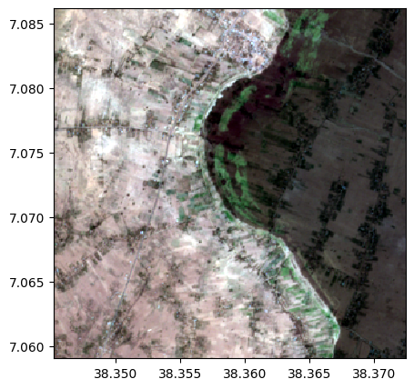
One can combine operations
names = {"CO" : 1,"B": 2,"G":3,"R":4,"RE1":5,"RE2":6,"RE3":7,"NIR":8,"WA":9,"SWIR1":10,"SWIR2":11,"SWIR3":12}
image_names=rastereasy.open(name_im,names=names)
image_names.info()

image_modified=image_names.crop(area=((50,100),(120,300))).resample(30).reproject("EPSG:27700")
image_modified.colorcomp()
image_modified.info()
- Size of the image:
   - Rows (height): 1000
   - Cols (width): 1000
   - Bands: 12
- Spatial resolution: 10.0  meters / degree (depending on projection system)
- Central point latitude - longitude coordinates: (7.04099599, 38.39058840)
- Driver: GTiff
- Data type: int16
- Projection system: EPSG:32637
- Nodata: -32768.0

- Given names for spectral bands:
   {'CO': 1, 'B': 2, 'G': 3, 'R': 4, 'RE1': 5, 'RE2': 6, 'RE3': 7, 'NIR': 8, 'WA': 9, 'SWIR1': 10, 'SWIR2': 11, 'SWIR3': 12}
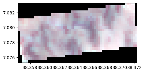
- Size of the image:
   - Rows (height): 23
   - Cols (width): 61
   - Bands: 12
- Spatial resolution: 39.353156172510154  meters / degree (depending on projection system)
- Central point latitude - longitude coordinates: (7.07928894, 38.36432299)
- Driver: GTiff
- Data type: int16
- Projection system: EPSG:27700
- Nodata: -32768.0

- Given names for spectral bands:
   {'CO': 1, 'B': 2, 'G': 3, 'R': 4, 'RE1': 5, 'RE2': 6, 'RE3': 7, 'NIR': 8, 'WA': 9, 'SWIR1': 10, 'SWIR2': 11, 'SWIR3': 12}
Some general functions
Sum, product, comparison, …
Weighted sum of images
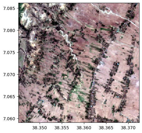
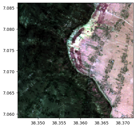
# 1. Read and plot two images
name_im1='./data/demo/im1.tif'
name_im2='./data/demo/im2.tif'

image1=rastereasy.open(name_im1)
image2=rastereasy.open(name_im2)
image1.colorcomp([4,3,2])
image2.colorcomp([4,3,2])
# Compute a weighted sum
weighted1=3
weighted2=5

image_sum=(weighted1*image1+weighted2*image2)/(weighted1+weighted2)
image_sum.info()
image_sum.colorcomp([4,3,2])
- Size of the image:
   - Rows (height): 300
   - Cols (width): 300
   - Bands: 12
- Spatial resolution: 10.0  meters / degree (depending on projection system)
- Central point latitude - longitude coordinates: (7.07261482, 38.35885970)
- Driver: GTiff
- Data type: float64
- Projection system: EPSG:32637
- Nodata: -32768.0

- Given names for spectral bands:
   {'1': 1, '2': 2, '3': 3, '4': 4, '5': 5, '6': 6, '7': 7, '8': 8, '9': 9, '10': 10, '11': 11, '12': 12}
Multiplication, division
# Multiplication of images
image_product = image1*image2
image_product.info()
image_product.colorcomp([4,3,2])
- Size of the image:
   - Rows (height): 300
   - Cols (width): 300
   - Bands: 12
- Spatial resolution: 10.0  meters / degree (depending on projection system)
- Central point latitude - longitude coordinates: (7.07261482, 38.35885970)
- Driver: GTiff
- Data type: float64
- Projection system: EPSG:32637
- Nodata: -32768.0

- Given names for spectral bands:
   {'1': 1, '2': 2, '3': 3, '4': 4, '5': 5, '6': 6, '7': 7, '8': 8, '9': 9, '10': 10, '11': 11, '12': 12}
# Division of images
image_divide = image1/image2
image_divide.info()
image_divide.colorcomp([4,3,2])
- Size of the image:
   - Rows (height): 300
   - Cols (width): 300
   - Bands: 12
- Spatial resolution: 10.0  meters / degree (depending on projection system)
- Central point latitude - longitude coordinates: (7.07261482, 38.35885970)
- Driver: GTiff
- Data type: float64
- Projection system: EPSG:32637
- Nodata: -32768.0

- Given names for spectral bands:
   {'1': 1, '2': 2, '3': 3, '4': 4, '5': 5, '6': 6, '7': 7, '8': 8, '9': 9, '10': 10, '11': 11, '12': 12}
Clip values
print(f'min max values before clip : {image.min()}, {image.max()}')
image_clip= image.clip(100,5000)
print(f'min max values before clip : {image_clip.min()}, {image_clip.max()}')
min max values before clip : 93, 5566
min max values before clip : 100, 5000
# this can also be done in inplace mode :
print(f'min max values before clip : {image.min()}, {image.max()}')
image.clip(100,5000, inplace=True)
print(f'min max values after clip : {image.min()}, {image.max()}')
min max values before clip : 93, 5566
min max values after clip : 100, 5000
Compute ndvi
name_im='./data/demo/im2.tif'
image=rastereasy.open(name_im)
# Get nir band (number 8)
nir = image.select_bands(8)
# Get red band (number 4)
red = image.select_bands(4)
# Compute ndvi
ndvi=(nir-red)/(nir+red)
# check info
ndvi.info()
# plot
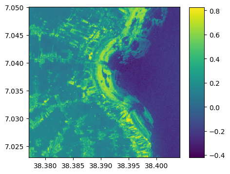
ndvi.visu(colorbar=True)
# Note : ndvi.colorcomp() works also
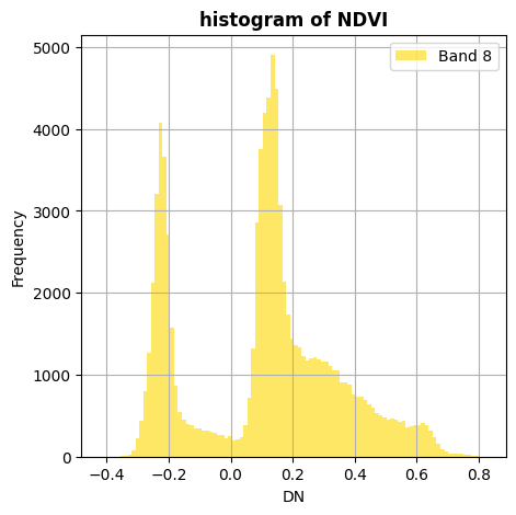
ndvi.hist(title='histogram of NDVI')
- Size of the image:
   - Rows (height): 300
   - Cols (width): 300
   - Bands: 1
- Spatial resolution: 10.0  meters / degree (depending on projection system)
- Central point latitude - longitude coordinates: (7.03647565, 38.39059829)
- Driver: GTiff
- Data type: float64
- Projection system: EPSG:32637
- Nodata: nan

- Given names for spectral bands:
   {'8': 1}
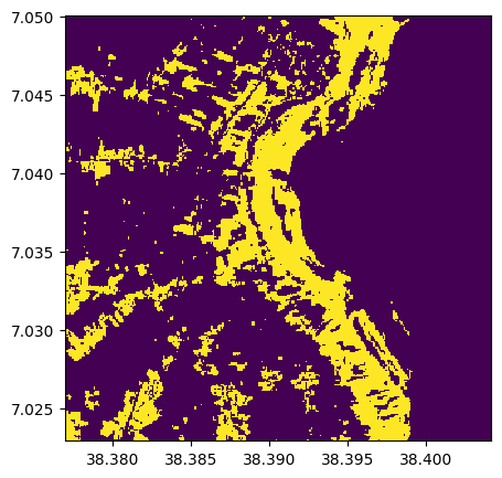
Identifying vegetation with (use >, <)
threshold=0.3
veget=ndvi>=threshold
veget.info()
veget.visu()
- Size of the image:
   - Rows (height): 300
   - Cols (width): 300
   - Bands: 1
- Spatial resolution: 10.0  meters / degree (depending on projection system)
- Central point latitude - longitude coordinates: (7.03647565, 38.39059829)
- Driver: GTiff
- Data type: bool
- Projection system: EPSG:32637
- Nodata: 0

- Given names for spectral bands:
   {'8': 1}
Identifying vegetation with ndvi.where() (similar than with numpy)
ndvi.info()
veget=ndvi.where(ndvi>=threshold,1,0)
veget.info()
veget.visu()
- Size of the image:
   - Rows (height): 300
   - Cols (width): 300
   - Bands: 1
- Spatial resolution: 10.0  meters / degree (depending on projection system)
- Central point latitude - longitude coordinates: (7.03647565, 38.39059829)
- Driver: GTiff
- Data type: float64
- Projection system: EPSG:32637
- Nodata: nan

- Given names for spectral bands:
   {'8': 1}
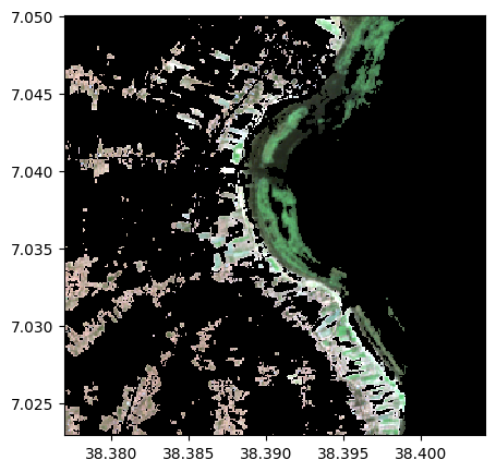
Identifying vegetation with indexing
image2=image.copy()
image2[veget==0]=0
image2.colorcomp([4,3,2])
Min, max of the image, per band, row, …
help(image.min)
print('Overall minimum of the image : ',image.min(),'\n')
help(image.max)
print('Maximum  of the image for each band: ', image.max(axis = 'pixel'),'\n')
help(image.std)
Help on method min in module rastereasy:

min(axis=None) method of rastereasy.Geoimage instance
    Calculate the minimum value along a specified axis.

    Parameters
    ----------
    axis : {'band', 'row', 'col', None}, optional
        The axis along which to compute the minimum:
        - 'band': Minimum across spectral bands for each pixel
        - 'row': Minimum across rows (lines) for each band and column
        - 'col': Minimum across columns for each band and row
        - 'pixel': Minimum across pixels for each bands
        - None: Global minimum of the entire image
        Default is None.

    Returns
    -------
    float or numpy.ndarray
        - If axis=None: A single value representing the global minimum
        - If axis='band': Array with shape (nb_rows,nb_cols) containing  mins along bands
        - If axis='row': Array with shape (nb_bands,nb_cols) containing mins along rows
        - If axis='col': Array with shape (nb_bands,nb_rows) containing  mins along cols
        - If axis='pixel': Array with shape (nb_bands) containing  mins along all pixels for each band

    Raises
    ------
    ValueError
        If an invalid axis is specified

    Examples
    --------
    >>> min_value = image.min()  # Global minimum value
    >>> print(f"Minimum pixel value: {min_value}")
    >>>
    >>> band_mins = image.min(axis='pixel')  # Minimum along all pixels for each band

Overall minimum of the image :  92

Help on method max in module rastereasy:

max(axis=None) method of rastereasy.Geoimage instance
    Calculate the maximum value along a specified axis.

    Parameters
    ----------
    axis : {'band', 'row', 'col', None}, optional
        The axis along which to compute the maximum:
        - 'band': Maximum across spectral bands for each pixel
        - 'row': Maximum across rows (lines) for each band and column
        - 'col': Maximum across columns for each band and row
        - 'pixel': Maximum across pixels for each bands
        - None: Global maximum of the entire image
        Default is None.

    Returns
    -------
    float or numpy.ndarray
        - If axis=None: A single value representing the global maximum
        - If axis='band': Array with shape (nb_rows,nb_cols) containing  max along bands
        - If axis='row': Array with shape (nb_bands,nb_cols) containing max along rows
        - If axis='col': Array with shape (nb_bands,nb_rows) containing  max along cols
        - If axis='pixel': Array with shape (nb_bands) containing  maxs along all pixels for each band

    Raises
    ------
    ValueError
        If an invalid axis is specified

    Examples
    --------
    >>> max_value = image.max()  # Global maximum value
    >>> print(f"Maximum pixel value: {max_value}")
    >>>
    >>> band_maxs = image.max(axis='pixel')  # Maximum along all pixels for each band

Maximum  of the image for each band:  [1438 2290 2478 2680 2958 4702 5118 5352 5281 4455 4268 3839]

Help on method std in module rastereasy:

std(axis=None) method of rastereasy.Geoimage instance
    Calculate the standard deviation along a specified axis.

    Parameters
    ----------
    axis : {'band', 'row', 'col', None}, optional
        The axis along which to compute the standard deviation:
        - 'band': Std dev across spectral bands for each pixel
        - 'row': Std dev across rows (lines) for each band and column
        - 'col': Std dev across columns for each band and row
        - 'pixel': Std dev across pixels for each bands
        - None: Global standard deviation of the entire image
        Default is None.

    Returns
    -------
    float or numpy.ndarray
        - If axis=None: A single value representing the global std
        - If axis='band': Array with shape (nb_rows,nb_cols) containing  std along bands
        - If axis='row': Array with shape (nb_bands,nb_cols) containing std along rows
        - If axis='col': Array with shape (nb_bands,nb_rows) containing  std along cols
        - If axis='pixel': Array with shape (nb_bands) containing  std along all pixels for each band

    Raises
    ------
    ValueError
        If an invalid axis is specified

    Examples
    --------
    >>> std_value = image.std()  # Global standard deviation
    >>> print(f"Standard deviation of pixel values: {std_value}")
    >>>
    >>> band_stds = image.std(axis='pixel')  # Standard deviation along all pixels for each band
# Extract the 30th line
image[30,:]
array([[ 933,  933,  933, ...,  221,  221,  221],
       [1278, 1250, 1254, ...,  284,  271,  252],
       [1678, 1624, 1664, ...,  456,  453,  448],
       ...,
       [2828, 2828, 2828, ...,  209,  209,  209],
       [3710, 3614, 3614, ...,  193,  193,  191],
       [3570, 3470, 3470, ...,  169,  169,  161]],
      shape=(12, 300), dtype=int16)
# all spectral values in a given pixel
row=20
col=10
print('spectral values in',row,',',col,' : ',image[row,col])
print('size of all spectral values in row',row,':', image[row,:].shape)
print('size of all spectral values in col',col,':', image[:,col].shape)
# check consistency
pixel_row = 15
pixel_col = 22
print('diff with table with values at row ',row,' in pixel col',pixel_col,':', image[row,:][:,pixel_col]-image[row,pixel_col])
print('diff with table with values at col ',col,' in pixel row',pixel_row,':', image[:,col][:,pixel_row]-image[pixel_row,col])
spectral values in 20 , 10  :  [ 986 1254 1582 2088 2317 2445 2552 2646 2729 2727 3543 3365]
size of all spectral values in row 20 : (12, 300)
size of all spectral values in col 10 : (12, 300)
diff with table with values at row  20  in pixel col 22 : [0 0 0 0 0 0 0 0 0 0 0 0]
diff with table with values at col  10  in pixel row 15 : [0 0 0 0 0 0 0 0 0 0 0 0]
# Csmall modifications
im1=rastereasy.open('./data/demo/sentinel.tif')
im2=rastereasy.open('./data/demo/sentinel.tif')+4
print((im2-im1).mean())
4.0